Project 1 - Health in the USA

By Devin Harris

Motivation

The motivation for this project was to illustrate potential correlations and trends between different economic, environmental, behavioral, demographic, and health related factors across all the U.S. counties. The goal of the project was to help people understand how these factors can influence each other while also providing quantitative data to each U.S. County.

Another source of motivation for this project was to get accustomed to the d3js library. This library helps aid in creating various charts through the use of dynamically created svgs. This library is heavily used in the CS 5124 - VISUAL INTERFACES DATA course which I took in my senior year and thus where this project stemmed from.

The Data

The data behind this project was pulled from the US heart and stroke atlas (https://www.cdc.gov/dhdsp/maps/atlas/index.htm) and was represented by a csv with attributes cnty_fips, display_name, poverty_perc, median_household_income, education_less_than_high_school_percent, air_quality, park_access, percent_inactive, percent_smoking, urban_rural_status, elderly_percentage, number_of_hospitals, number_of_primary_care_physicians, percent_no_heath_insurance, percent_high_blood_pressure, percent_coronary_heart_disease, percent_stroke, percent_high_cholesterol per U.S. county.

You can download the data here to see for yourself!

Download

Sketches

I made the following sketches at the beginning of this project to help illustrate how I could visually represent this data in an easy-to-understand way.

* Sketch 1 *
* Sketch 2 *

The first sketch above was a first pass at how I could organize the data into various chart types. You can see ideas around showing a circle for every county in a scatter plot, showing 2 bars for each county (1 bar for each attribute selected) in a bar chart, side by side choropleth maps, and even bar charts based on percentage ranges and county count on the y axis were some ideas I had originally.

The second sketch was a refinement on the ideas put forth in the first sketch. In the second sketch you can see I pulled out some common controls like attribute selection, chart type selection and even started lofting the idea of aggregation selections into a left hand side form panel. Then I would have the right hand side show 1 chart at a time, possibly even using a carousel type interaction for switching between chart types. This of course is still a little off from my final version but ideas from this sketch were very closely followed in the final implementation.

Gui

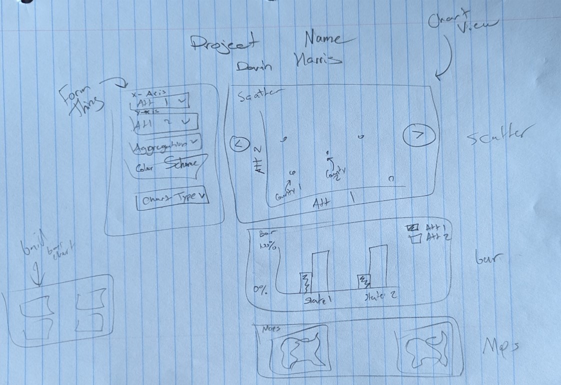
The above sketches then translated to the actual visualization of these components in my app gui.

As you can see there are 3 different views (1 for each chart type). I then have a global form on the left-hand side that provides attribute changing, grouping/aggregating, and in some cases sorting functionality. I wanted to make these controls shared between the different chart types as much as possible to make switching between them feel more fluid and keeping the same selections between charts. 
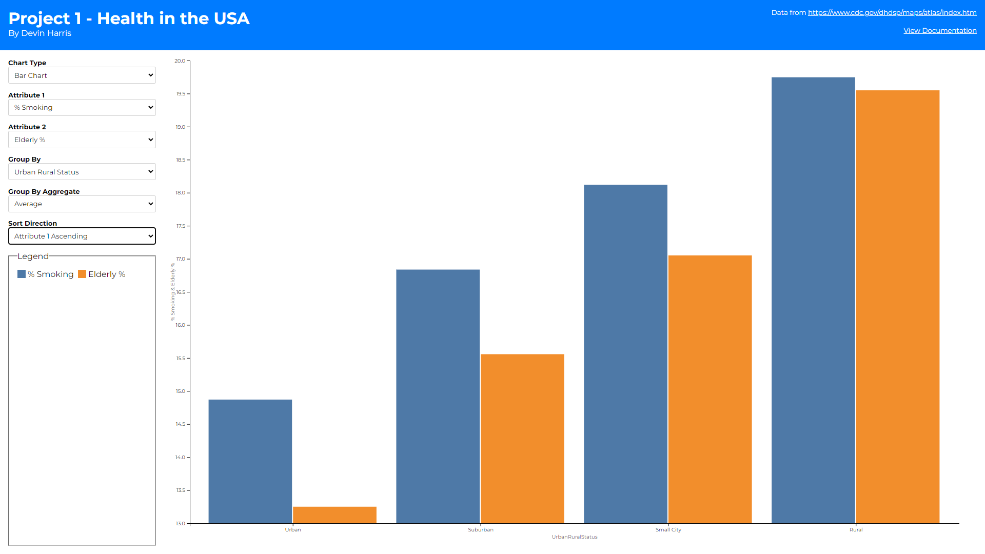
The most interesting thing about this form section to me is the grouping functionality. Upon looking at the data I found that showcasing datapoints for all 3000+ counties would be difficult in some cases. Thus, I wanted a way to limit the number of datapoints for these instances. By grouping all the counties into their respective state, or urban rural status I can reduce the number of datapoints to render dramatically. This led to the question of how should I group them? Should I average all the datapoints together? Take the maximum value? This is where the group by aggregate selection came in. This allows users to not only group datapoints together but decide how to aggregate the values of that group as well.

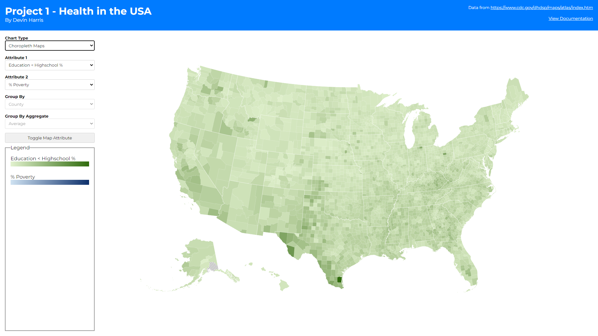
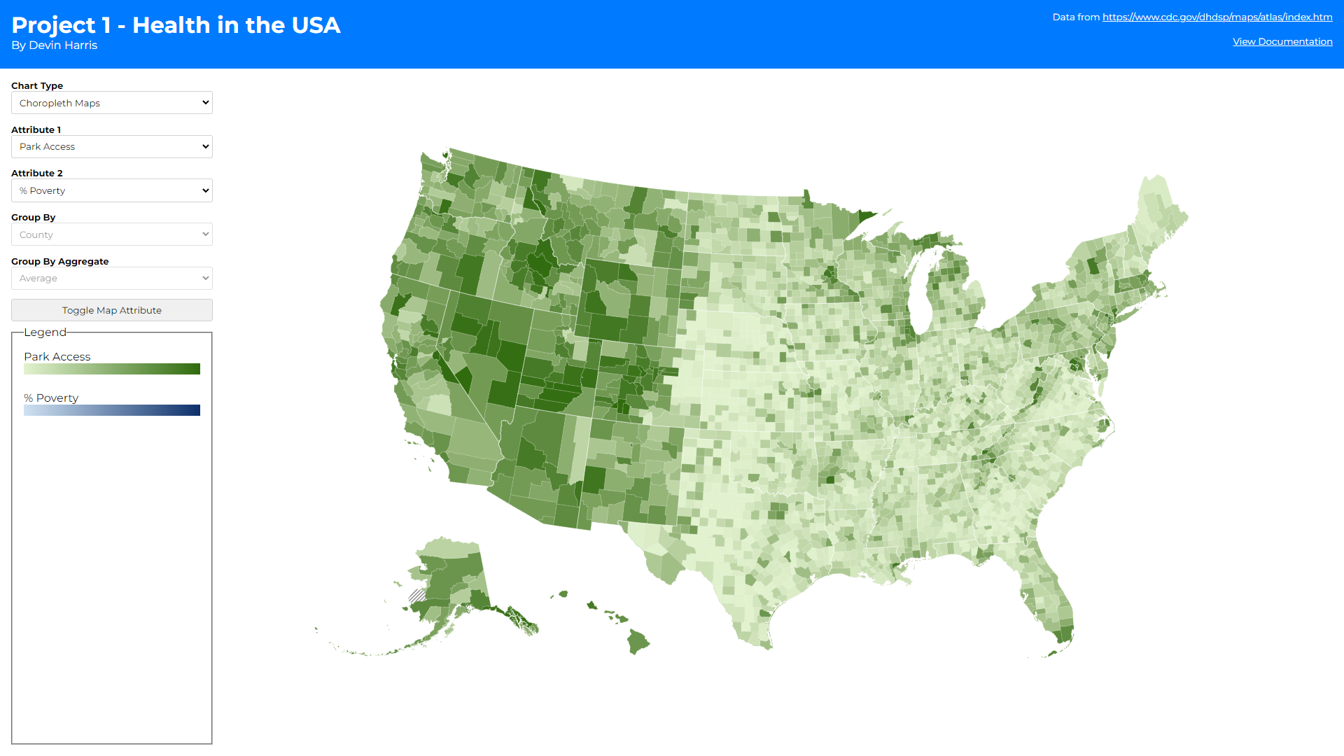
You may also notice there are some additional controls when the bar and choropleth maps are selected. At first, I wanted to display two maps side by side (1 for each attribute) but quickly realized that horizontal scroll would be needed to do this and comparing over scroll felt incorrect. Thus, I opted to add more controls on the right-hand side to allow the user to toggle how the coloring is applied to a single map (based on the first or second attribute depending on how many times the toggle button is clicked). This prevents the user from having to sift their eyes across two different maps when they want to compare those hot/low spots I mentioned above, while also giving more screen real estate to the map.

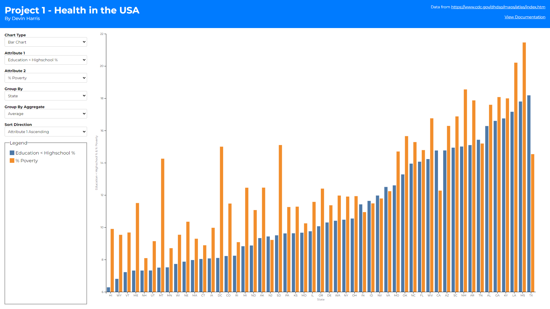
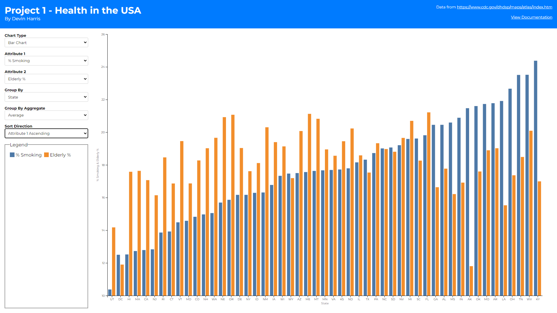
  • The first is a sorting selector on the bar chart. This was created to help assess the overall trend of the data. Assessing which county/state has the highest/lowest value in the bar chart was difficult before this selector. With it, sorting allows you to pull the highest or lowest values to the left most points on the graph which also help show the general slopes of whichever attribute you are sorting over. Alphabetical sorting also helps users find a specific county/state/urban rural status they are looking for without having to scroll blindly. It also allows for comparing the growth/decay over two attributes to help identify if there is some correaltion between them.
  • The second is a toggle button on the chorpleth map.

There is also a legend section to help illustrate what colors line up to what groups or values, again depending on chart type. The legend can also help with filtering down the dataset as well. Clicking a color swatch with show/hide that group from the chart making it easier to hide outliers. The following rules were followed for this legend and color scheme building within the charts:

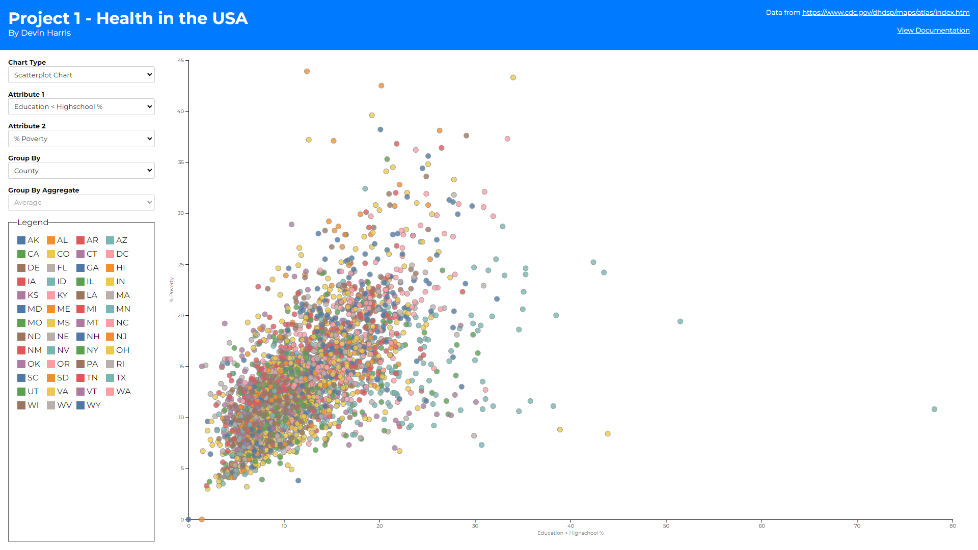
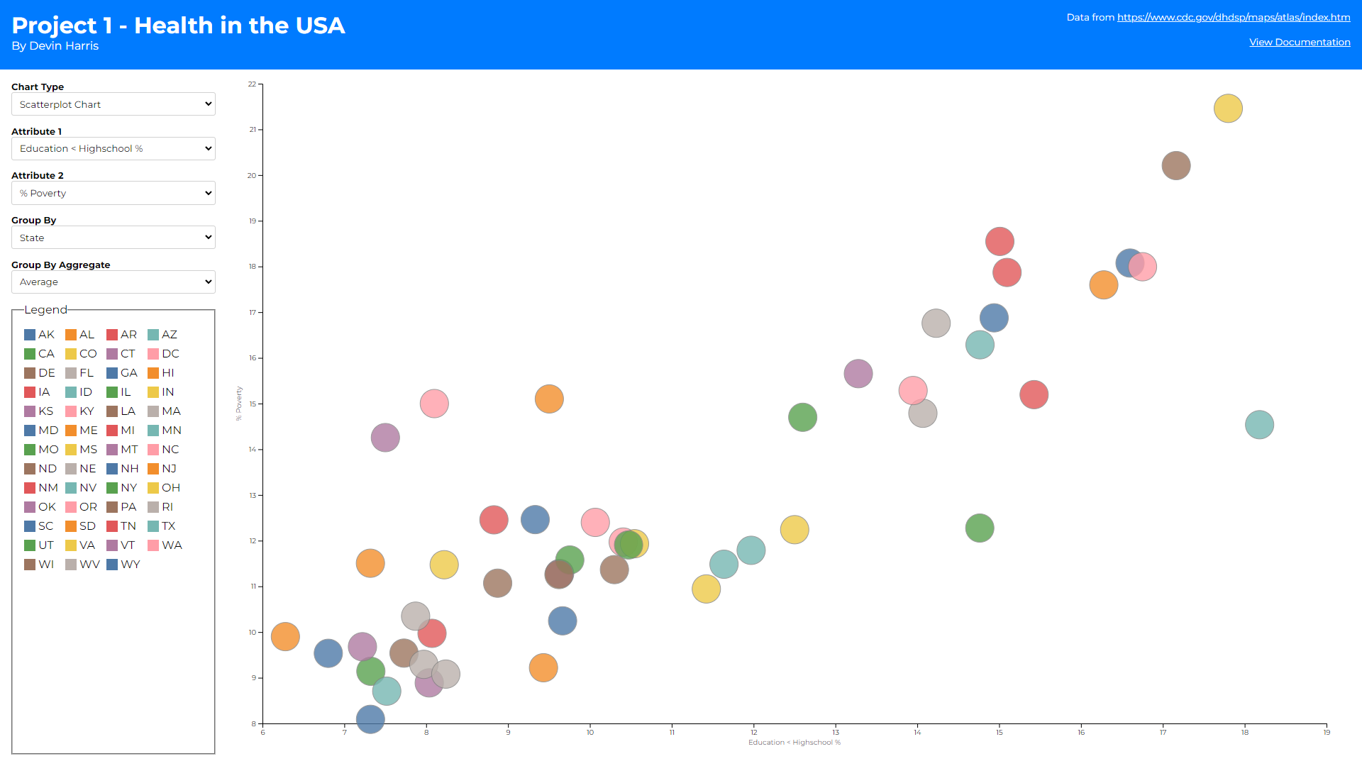
  • Scatter plots color their dots based on the state if the group by is county or state. This is because a legend with a color for every county was hard to sift through and did not seem to help the visualization. If group by is urban-rural-status the 4 statuses are used as the legend domain.
  • Bar charts color their bars based on attribute. I decided to show bar charts as two bars per x axis tick because it helped to compare the two attributes per county/state/urban-rural-status easier. This of course led me towards keeping the colors consistent between attributes to better showcase how they compare across different points on the x-axis.
  • Choropleth maps used a green and blue sequential scale for the 1st and 2nd attribute selected respectively. This helps differentiate the two maps without having to label which map is showing which attribute while also showing the geographical hotspots/lowspots for each attribute across the United States.

Finally, there are some interesting interactions that can be made within these charts. Brushing to select certain datapoints is possible on the scatter plot chart. These selections are highlighted across the other chart types as well. Brushing was difficult to implement in the bar chart because zooming and panning was incorporated there. This was partly because when grouping by counties, in most cases there is not enough space to assign at least 1 pixel to every bar chart, so allowing the user to zoom in was necessary to get any use out of the bar chart on that group by. This zooming conflicted with the brushing implementation so the bar just shows selections made from other graphs instead. The choropleth map also had a brushing problem, but selecting can still be done from this chart. Simply clicking on a county will toggle its selected state and that will propogate across the other charts as well.
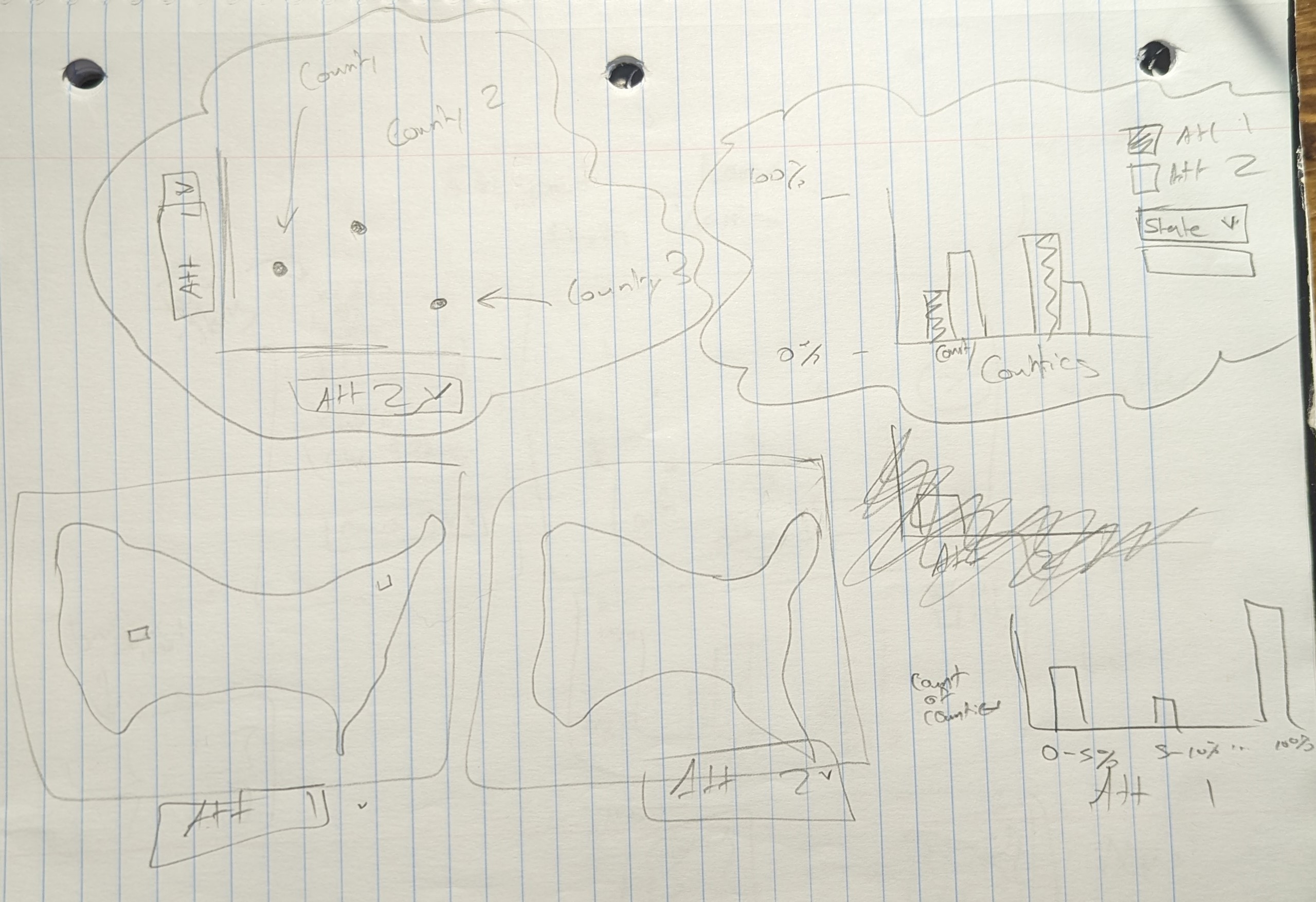
Discovery

There were tons of findings you can discover with this application. Here are some interesting ones I found:

To the left I selected “Education < Highschool %” as my x-axis and “Poverty %” as my y axis. Grouping by state we then see that on average the more people with less than high school education the more people there are in poverty (in general)

Above we first see that the average “% of smokers” per state does not really translate to the average “Elderly %” per state. I half expected some correaltion because smoking (at least in my opinion) doesn't seem as common with my peers as I perceived it to be in say my parents generation.

This lead me to group by urban rural status instead (shown in second screenshot). With that grouping there is a definite correlation suggesting the more rural you get not only the more smokers there are, but the more elderly there are to.

And finally, to the left I wanted to view park access across the United States. You can see a substantially shift as you enter the west where the west has way more park access than the east (again in general). I was not able to find another attribute that followed this trend. Maybe if our dataset had more information on say population density, or temperature readings, a correlation between park access and those attributes could shed light on this phenomenon.

Future Works

There are some improvements I would liked to have made to this project given I had the time. Firstly, I would have liked to improve the brushing/selection I did on the scatter plot with the other charts. My main question on I kept trying to answer was how would changing the group by selection affect the selection. If I had counties selected, then switched to selecting states I would probably have to clear the previous selection which I haven’t decided if I’m ok with thus why I didn’t fully opt into that on the other graphs where brushing was already problematic.

I also would have liked to improve the bar chart when grouping by counties. There are so many counties that without zooming in the bar chart is pretty much useless with that grouping. Possibly having a secondary area chart to replace the zooming/panning logic could open up more options especially around brushing that I mentioned above. Here was an example of this that I tried implementing but was unsuccessful in the end: Link

Process

For this project I used d3, plain javascript, html, and css. I unfortunately was told things like svelte and typescript were not allowed late into the project. Reasons being for consistency between projects and other classmates. I however had made quite a bit of progress using those tools thus why if you look at the code there are a lot of svelte related snippets. Hopefully this does not detract from the project but the live versions code all exists within the "vanilla" folder within the linked repo.

The general approach I had was to define a "globals.js" file where all my shared variables (such as attributes selected, group by selected, etc...) could be defined. Then utilizing classes I created builders for various areas of my code. For example the form-builder.js is a class responsible for dynamically building all the controls (excluding the legend pieces which was done in the legend-builder) and listening the various change and input events on them. This form builder could then trigger updates on the global scatter, bar, and choro variables which themselves were set to instances of new scatter-builder, bar-builder, and choropleth-builder classes. This approach allowed for seperation of concerns while allowing interactions to be shared between charts.

You can run it by cloning the project, and opening the index.html with something like the "Live Server" extension in vscode.

Check out the links below to view the live site and code as well!

Live Site

Code

Demo Video